YOLOv3从前两代发展而来,融合了老式的YOLO系列的one-stage的特点和一些SOTA模型的tricks。要了解YOLOv3,最好是先读YOLOv1中关于回归概念和损失函数的描述,YOLOv2基本有了YOLOv3的形状但是还没有ResNet的思想,不如直接看YOLOv3。YOLOv3模型有这几大重点:
独特的网络结构Darknet-53。融合了BN,ResNet的shortcut,多尺度feature map的拼接;
多尺度的输出。输出是具有三个尺度的特征图的拼接,前代的小目标检测的弱点得到了克服;
SOTA的锚框方法。虽然是YOLOv2就有的,但是YOLOv3做了改进,anchor-based的方法成全了YOLOv3;
精心设计的损失函数。沿用YOLOv1对损失函数的定义,稍作调整。
README
- 这篇文章在英文版的review基础上修改得来,写的时候觉得之前review的是个什么东西,重点只把握一部分,没有认识到网络结构和损失函数的重要性。所以最后文章把原文放底下,细节算新写的。原文还是可以看的,当作熟悉整体思路,以及看YOLOv3的测试表现的描述。
- 理解YOLOv3重在理解网络结构的层,特别是检测层的功能。
- 我想的是,一定要展现YOLOv3为什么从YOLOv2能变强这么多,因为它俩实际上很像,但是些微的调整就带来了大的进步,ResNet的shortcut结构为什么能带来更好的特征描述,这些还要从ResNet讲起。话说我为什么要把残差网络当作我的第一篇review的论文...叫残暴起点算了。
- 文章里的很多东西,是论文里没写到的,细节一般来源于按照前人的from-scratch系列重写的代码。
- 引用很精彩,用来做扩展阅读挺好。
网络结构
这里我po出两张图,第一张是直观的,重在展现feature map的变化过程;第二张是细节的,重在展现网络的起作用的单元结构。
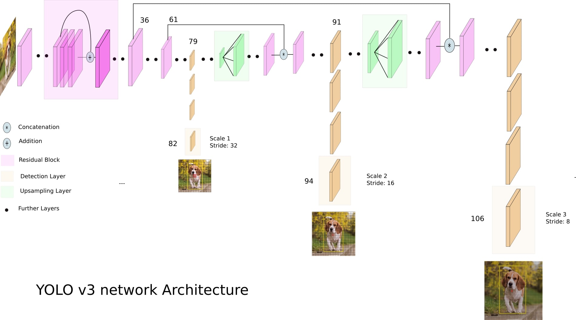 ◎ Image credit: https://towardsdatascience.com/yolo-v3-object-detection-53fb7d3bfe6b
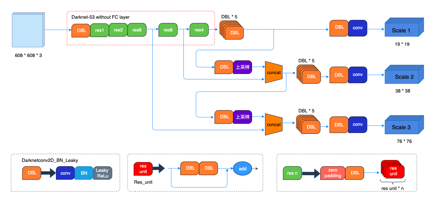 ◎ Image credit: https://blog.csdn.net/leviopku/article/details/82660381
- 没有池化层。那怎么实现特征图尺寸变换呢?是卷积核的stride的改变来实现缩小的。YOLOv3和YOLOv2一样,输入经过五次缩小缩小比例为$1/2^5=1/32$,所以要求输出是32的倍数。如果输入为416×416,则最小的特征图是13×13(考虑属性的维度则是13×13×255)的。
- 没有全连接层。那输出不是scores了吗?对的,one-stage的YOLOv3,将边界框的定位和目标的分类当作回归问题,融合为一步了,输出的tensor里,既包括所有候选的位置信息的预测,也包括平常情况下全连接层所输出的分类分数。
多尺度的输出
YOLOv3在feature map的每一个格子都会预测边界框。将目标的边界框的定位当作回归问题做,通过减小锚框和真实边界框的损失函数,学习预测锚框缩放大小和偏移。YOLOv3在一个特征图格子会预测三个候选框,multi-scale是通过三个拼接成的不同scale的特征图实现的,会有很多候选框,这三个scale是在网络中不同位置实现的。
检测层
检测层不同于传统的CNN中的层,使用的检测核为1×1×(B×(5+C))的,B是指特征图一个格子所能预测的边界框数目,5表示一个边界框的4个位置属性+一个目标分数,C是指类别数目。在COCO训练集上训练的YOLOv3里,B=3, C=80,所以检测核大小是1×1×255的。但是注意,虽然检测层有kernel的设定,但这样的设定更相当于一种等效,并没有规定是按照kernel运算的,而是将检测层输入(即前面的层的输出)调整维度,输出三维的tensor,也就是说这样的运算导致输出的tensor中每个格子会有255的深度。具体地,输入经过维度调整,
| |
👆Source permalink.
第一维表示图片的ID,大小是
batch_size;第二维是这张图片在这个scale的边界框ID,总数为此次feature map所有的边界框数目,即$n_{fm}\times n_{fm}\times B$;
第三维是所有的按顺序重排的一个边界框的所有属性项,总数是5+C=85=85。
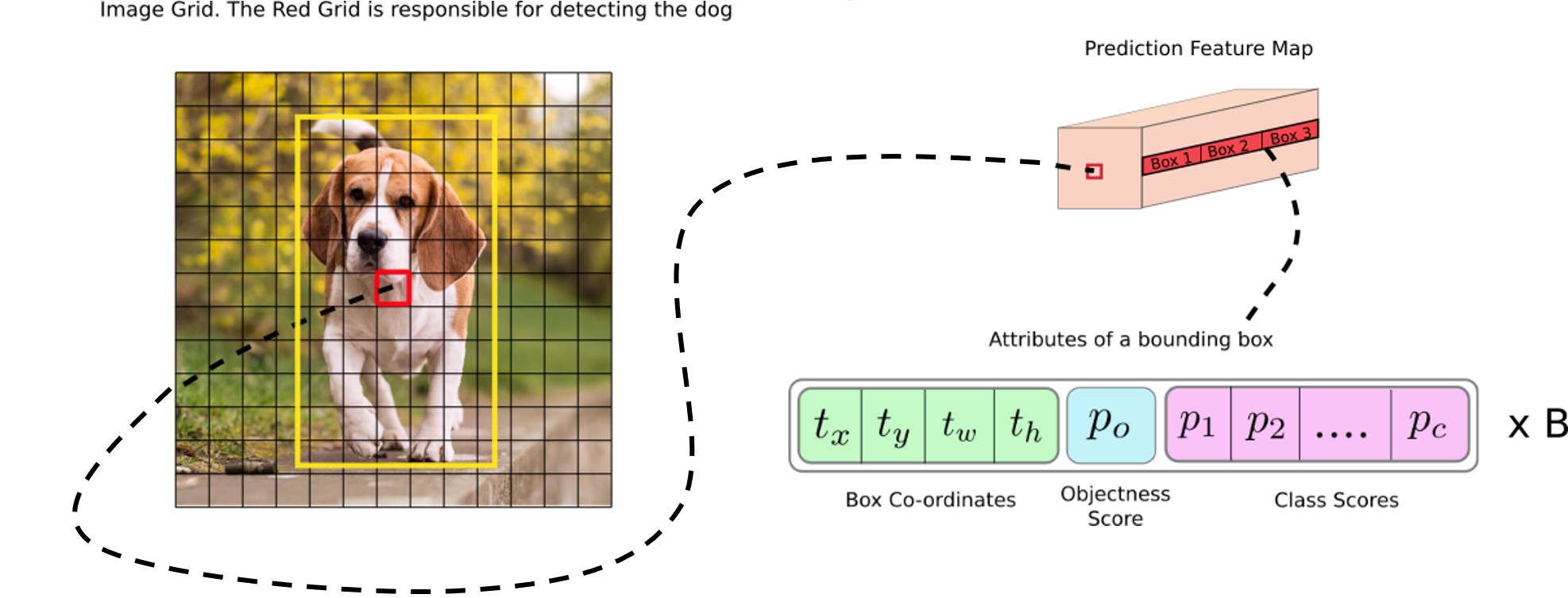 ◎ Credit: https://blog.paperspace.com/how-to-implement-a-yolo-object-detector-in-pytorch/
尺度变换
文章开头说到,YOLOv3的尺度变换不是通过池化层实现的,而是变换卷积层的stride做的。假设输入图片为416×416,YOLOv3在三个scale上做预测,预测的特征图结果按照32/16/8的倍数从原始图片下采样得来,即分别使用了32/16/8的stride,那么结果的特征图大小分别为13×13,26×26,52×52,每个格子预测3个边界框,总共: $$ (13\times 13+26\times 26+52\times 52)\times3=10647 $$
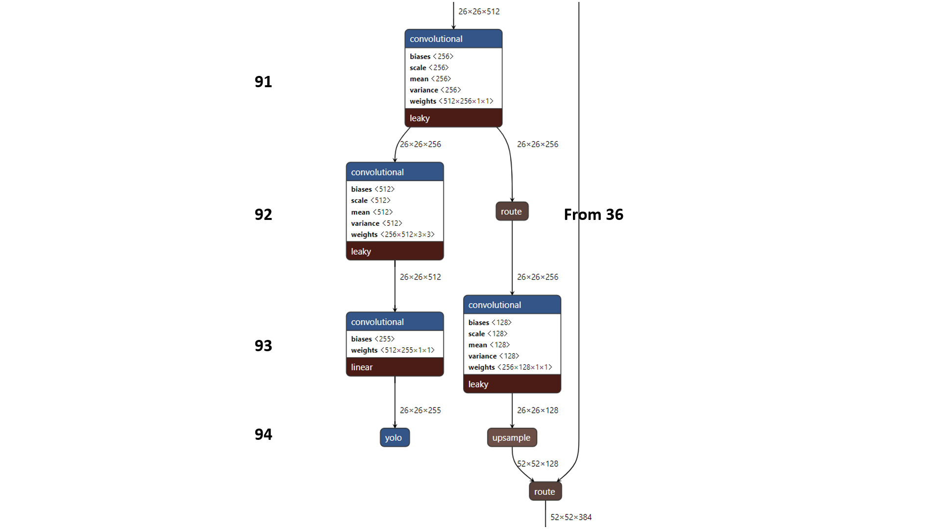
以下给出网络中实现三种尺度的特征图的位置的Netron图示:
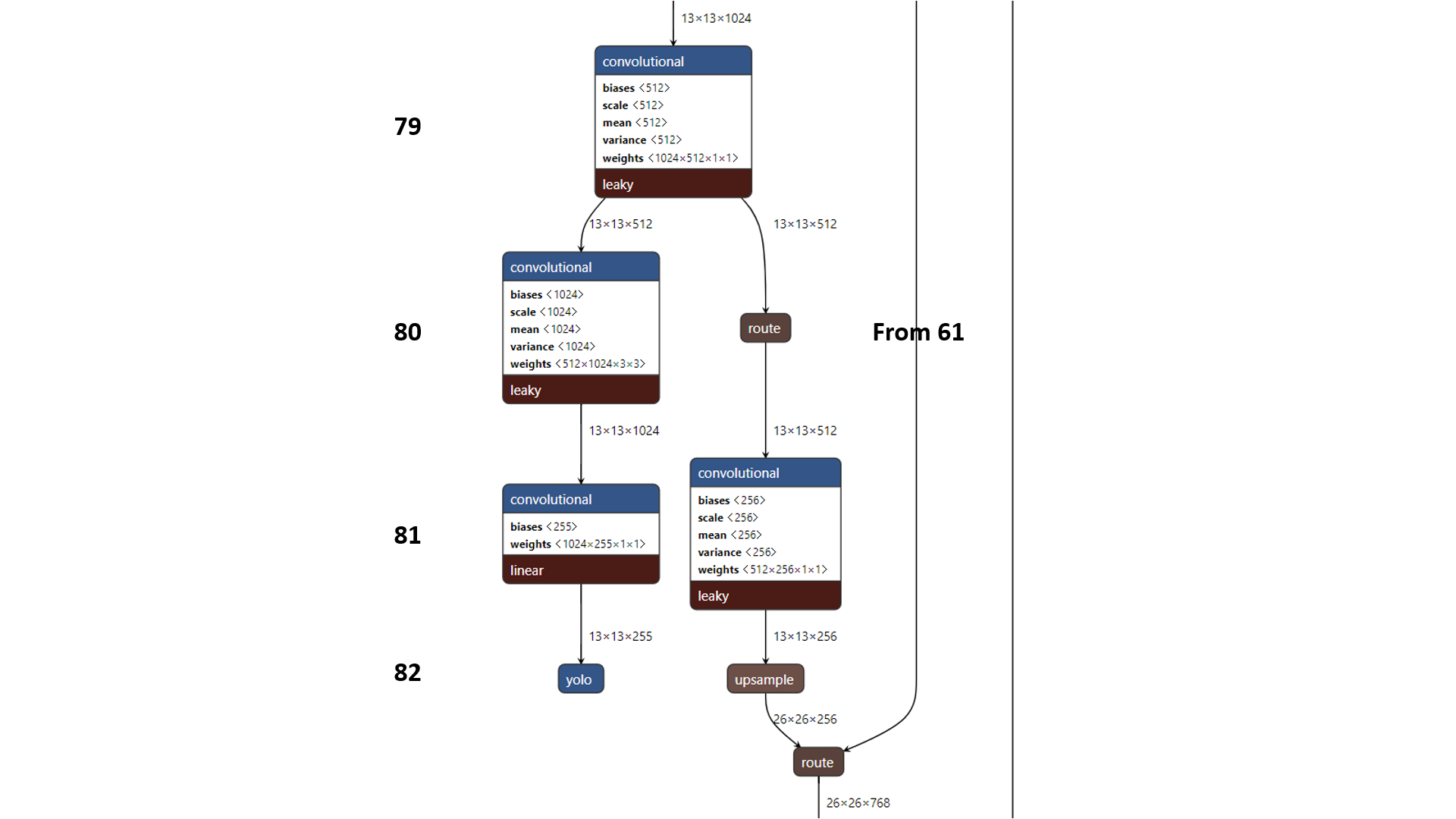 ◎ 第一次预测结果
 ◎ 第二次预测结果
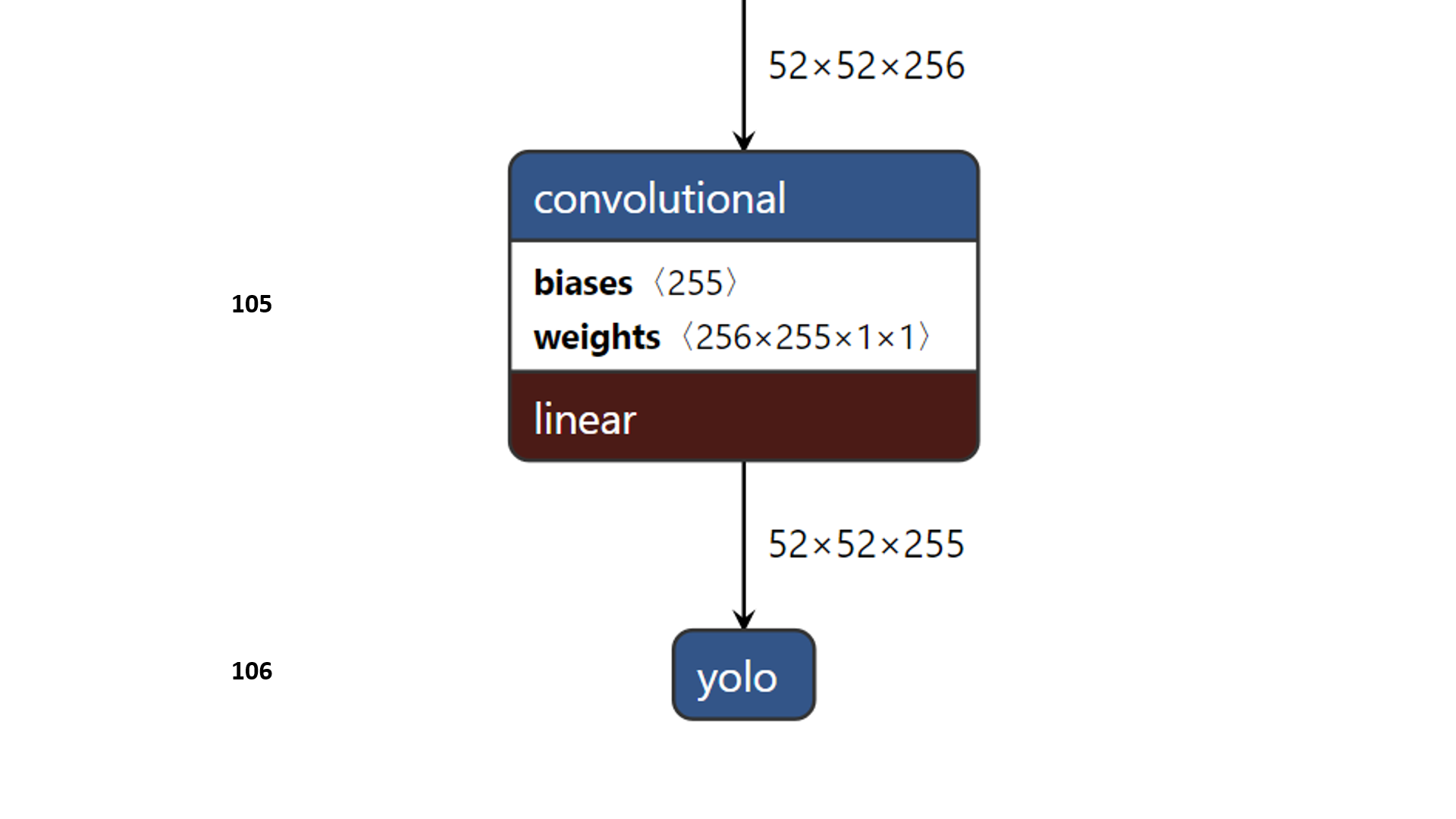 ◎ 第三次预测结果
锚框方法
边界框的预测使用到了上文所说的检测层三个尺度上的输出,他们包括了一幅图片三个尺度所有的候选,以及候选的位置信息,目标分数和分类分数,即:
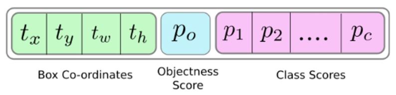 ◎ Bounding box attributes
**锚框(anchors)是一类设定好的先验框(priors),YOLOv3网络预测出对数空间上的转换关系,或者说是偏移,先验框因此转换为后验框,即候选。**这一句话有两个概念,第一个是锚框,YOLOv3定义了九个锚框,它们是在数据集上聚类得来的:
anchors = 10,13, 16,30, 33,23, 30,61, 62,45, 59,119, 116,90, 156,198, 373,326
这些数字表示锚框的尺寸,分别是宽度和高度。每一个尺度只用上三个锚框,前三个用于最大的特征图,即最后一个检测层,适合检测原图中小尺度的目标,中间三个用于中间的特征图,后三个用于最小的特征图,分别对应中间和第一个检测层,适合检测原图中中等和大尺度的目标。
第二个概念是转换关系。YOLO不预测边界框的绝对位置,而是相对于格子左上角的偏移。在转换之前,检测层把前面的输出先简单处理。把中心坐标用sigmoid函数规定到0-1上,目标分数也通过sigmoid函数激活,这样做是为了表示相对于格子左上角的偏移。
| |
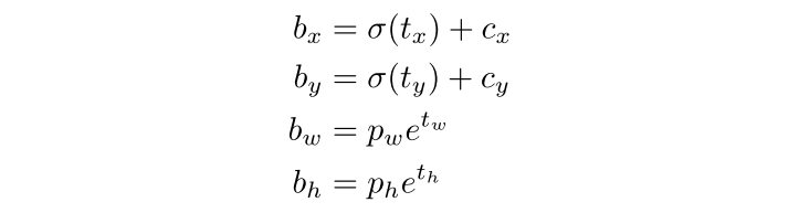
处理后的结果包括位置信息:$t_x,t_y,t_w,t_h$,目标分数$p_0$,以及分类分数。首先需要把网络输出转换为边界框中心坐标$b_x,b_y$和宽度$b_w$高度$b_h$的预测:
$$
\begin{aligned}
b_x&=\sigma(t_x)+c_x\\
b_y&=\sigma(t_y)+c_y\\
b_w&=p_we^{t_w}\\
b_h&=p_he^{t_h}
\end{aligned}
$$
其中$c_x,c_y$表示特征图格子左上角的坐标,$p_w,p_h$是锚框的尺寸。
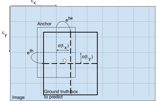 ◎ 转换到预测框
举个例子,对于13×13特征图的中间的格子,即左上角坐标为(6, 6),如果我们的中心坐标经过sigmoid之后为(0.4, 0.7),那么得到此候选在feature map上的中心坐标为(6.4, 6.7)。
至于目标分数和分类分数。前者用于Objectness thresholding,后者用于NMS,都是减少候选的操作,就不细讲了。
损失函数
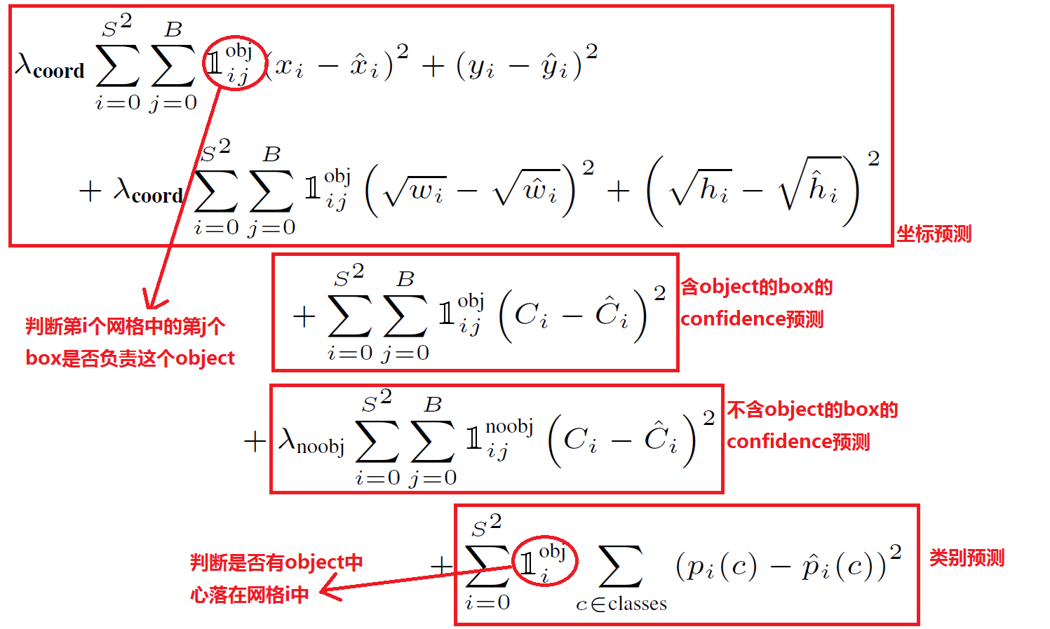
前代的损失函数全部采用Sum-squared Error Loss:
 ◎ Credit: https://blog.csdn.net/qq_30159015/article/details/80446363
- 第一行为总平方误差,是位置预测的损失函数;
- 第二行为根号总平方误差,是宽度和高度的损失函数;
- 第三,四行对目标分数或者置信度用总平方误差作为损失函数;
- 第五行对分类分数用总平方误差作为损失函数;
YOLOv3对后三行做了修改,将总平方误差替换为分类任务中更好用的交叉熵误差。也就是说,YOLOv3中的目标置信度和分类分数通过逻辑回归实现了。同时,每一个真实框,只匹配一个边界框,也就是IoU最大的那个。
细节和问题
不用softmax。前代的YOLO网络使用了softmax处理两种分数,但是这样做的前提是数据集的类是完全互斥的,也就是说目标如果属于A类,就不可能是B类,COCO满足这一条件。但是如果一个数据集有Person和Women这样的类别,这样的前提就不满足了,所以YOLOv3使用了逻辑回归来预测分数(或者说采用交叉熵loss),另外使用thresholding来预测一个目标的多个标签,而不是用softmax选分数最大的那个标签。
使用了更多的anchor。YOLOv2使用了5个anchors,而YOLOv3使用了9个。
offsets为什么constrain到[0, 1]上而不是[-1, 1]上?因为是采用对格子左上角的相对坐标,一个格子只管右下方的坐标就行。(issue)
从自己的数据集获取anchors。目标检测算法之YOLO系列算法的Anchor聚类代码实战。
预处理步骤。网络的输入是正方形的,所以得把图片处理成正方形的。代码是把图片按比例缩放,嵌入长边一致的正方形中,多余位置用padding。
引用
- Redmon, J. and Farhadi, A., 2018. Yolov3: An incremental improvement. arXiv preprint arXiv:1804.02767.
- Redmon, Joseph, et al. "You only look once: Unified, real-time object detection." Proceedings of the IEEE conference on computer vision and pattern recognition. 2016.
- Redmon, Joseph, and Ali Farhadi. "YOLO9000: better, faster, stronger." Proceedings of the IEEE conference on computer vision and pattern recognition. 2017.
- yolo系列之yolo v3【深度解析】
- 【目标检测】yolov3为什么比yolov2好这么多
- How to implement a YOLO (v3) object detector from scratch in PyTorch: Part 1
- What’s new in YOLO v3?
原文
Abstract
We present some updates to YOLO! We made a bunch of little design changes to make it better. We also trained this new network that's pretty swell. It's a little bigger than last time but more accurate. It's still fast though, don't worry. At 320 × 320 YOLOv3 runs in 22 ms at 28.2 mAP, as accurate as SSD but three times faster. When we look at the old .5 IOU mAP detection metric YOLOv3 is quite good. It achieves 57.9 AP 50 in 51 ms on a Titan X, compared to 57.5 AP 50 in 198 ms by RetinaNet, similar performance but 3.8× faster. As always, all the code is online at https://pjreddie.com/yolo/.
Aim
There is an unfinished issue existing in the second generation: poor performance in detection of small objects or detection of a group of small objects. The author managed to solve this issue and promote accuracy while still maintaining the speed of the model. He aimed to provide the information of what he made to make YOLOv2 better and how he did it.
Summary
The author first shared the tricks he used to improve the performance.
Bounding box prediction. YOLOv3 addresses the prediction of bounding boxes as a regression problem. The loss function is the MSE. And the gradient is the ground truth value minus the prediction: $\hat{t}_b-t_b$, where $t_b$ is the tensor of the coordinates for each bounding box. The tensor is used to calculate the predictions as:
The objectness score is 1 if the bounding box prior overlaps a ground truth object more than any other priors. If the box prior overlaps the ground truth by over 0.5 but is not the most, the prediction is not counted.
Class prediction. Each box now predicts the classes using multilabel classification. Softmax is substituted with binary cross-entropy loss function. This modification is suitable on more complex datasets. Softmax assumes that each class is independent while some dataset contains classes which are overlapping (like Woman and Person)
Prediction across scales. The author used a similar concept to SPP: adopting the feature extractor and the additional convolutional layers to encode a 3D tensor ($N\times N\times [3*(4+1+80)]$) prediction (at three scales) including the bounding box (4 coordinates), objectness (1 objectness score) and class predictions (80 classes). The algorithm takes the feature map from 2 layers previous and concatenates it with the $2\times$ unsampled feature map. This combined feature map is processed via a few more convolutional layers to predict a tensor at twice the size. The same process is applied to this tensor to create the third scaled feature map. Nine box priors and three scales are chosen via k-means clustering as before.
Feature extractor. The authors used a new but significantly larger network called Darknet-53. Darknet-53, compared to Darknet-19, adopts residual shortcut connections (ResNet). It is proved to yield state-of-the-art results: Similar performance to ResNet-152 but $2\times$ faster. Also, Darknet-53 can better utilize the GPU.
Training. They used multi-scale training instead of mining.
Then the author introduced some trials that didn't help.
- Anchor box x,y offset predictions. The linear activation of x,y offset as a multiple of the box width or height can decrease the stability.
- Linear x,y predictions instead of logistic functions lead to reduced mAP.
- Focal loss does not help improve the performance but drops the mAP.
- Dual IoU thresholds and truth assignment (Faster R-CNN) does not lead to good results.
Experiments are performed on COCO dataset. The model YOLOv3 is firstly trained on COCO trainset and then tested on the test set. Results indicate that YOLOv3 is comparable to SSD variants but $3\times$ faster, but behind the RetinaNet. However, YOLOv3 achieve state-of-the-art performance at .5IOU metric. In terms of small object detection, YOLOv3 performs better via multis-scale predictions but is worse while detecting larger objects.
Comments
My thoughts
The good side is: The paper presents explicit knowledge about what factors contributes to the improvements in YOLOv3's performance. The sections are easy to follow and understand. But compared to the paper of YOLOv2, this paper is less rigorous and precise.
- The authors revealed that he took the tables of performances of backbones from other research instead of reproducing and experimenting them uniformly.
- The authors didn't present all trials they made that failed but the things that they can remember. We may lack information of some potential but crucial issues that leads to poor performance.
Comparison
The paper in particular demonstrates the results of the performance at .5IOU metric. The best YOLOv3 model achieved state-of-the-art trade-off between accuracy and speed. It achieves 57.9 $AP_{50}$ in 51 ms on a Titan X, in contrast to 57.5 $AP_{50}$ in 198ms by RetinaNet. YOLOv3 was still not the most accurate detector but the most balanced and the fastest detector at that time.
Applications
Similar to YOLOv2, YOLOv3 can be used as the state-of-the-art detector at high FPS in high resolutions. However, in low resolutions or the cased when top accuracy is not necessary, YOLOv2 is much better because Darknet-19 can run at 171 FPS tested with $256\times 256$ input images compared to 78 by Darknet-53. The authors, in particular, addressed this issue, and they demonstrated that distinguishing an IOU of 0.3 from 0.5 is hard for humans. So for machines, .5IOU metric is also enough in object detection.