The task is to write my own codes to learn a decision tree using two features (the souce clusters and the destination clusters) to predict the classification field. Therefore, the first thing step is to read cluster dataset with classification labels. Some samples of the dataset are shown in the table below:
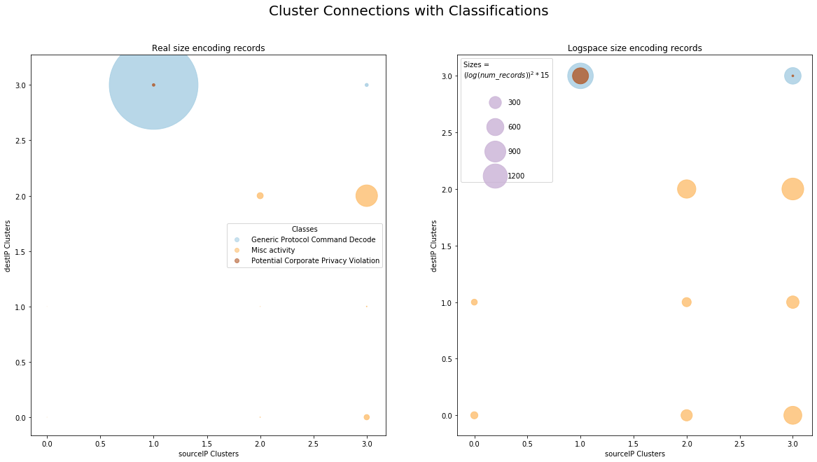
Before learning the decision tree, a similar size-encoding scatter graph is generated to demonstrate what classes that the points (different kinds of communications) will belong to. In the scatter graph, points of the same class will be drawn in the same color. See Figure
classes=cluster_data['class']# Extract the class columnunique_classes=np.unique(classes)# Unique classes# Replace the string names with the indices of them in unique classes arraycluster_data_digit_cls=cluster_data.copy(deep=True)fori,labelinenumerate(unique_classes):cluster_data_digit_cls=cluster_data_digit_cls.replace(label,i)print('Cluster dataset with indices as class names generated:\n',cluster_data_digit_cls.head())# Generate triples with indices of sourceIP cluster, destIP cluster and classcluster_triples=[(cluster_data_digit_cls.iloc[i][0],cluster_data_digit_cls.iloc[i][1],cluster_data_digit_cls.iloc[i][2])foriincluster_data_digit_cls.index]# Use Counter methodcounter_relation=Counter(cluster_triples)# Generate the numpy array in shape (n,4) where n denotes all types of triples and the four column contains the number of records of the corresponding triples. This step may cost about 10 secondsrelation=np.concatenate((np.asarray(list(counter_relation.keys())),np.asarray(list(counter_relation.values())).reshape(-1,1)),axis=1)# Save the dataset with counts# pd.DataFrame(relation, columns=['sourceIP cluster', 'destIP cluster', 'class', 'counts']).to_csv('relation.csv')# Generate data for size-encoding scatter plotx=relation[:,0]# Source IP cluster indicesy=relation[:,1]# Destination IP cluster indicesarea=(relation[:,3])**2/10000# Marker size with real number of recordslog_area=(np.log(relation[:,3]))**2*15# Constrained size in logspacecolors=relation[:,2]# Colours defined by classes# Create new subplots figurefig,axes=plt.subplots(1,2,figsize=(20,10))fig.suptitle('Cluster Connections with Classifications',fontsize=20)plt.setp(axes.flat,xlabel='sourceIP Clusters',ylabel='destIP Clusters')# Scatter plot: use alpha to increase transparencyscatter=axes[0].scatter(x,y,s=area,c=colors,alpha=0.8,cmap='Paired')axes[0].set_title('Real size encoding records')# Legend of classeshandles,_=scatter.legend_elements(prop='colors',alpha=0.6)lgd2=axes[0].legend(handles,unique_classes,loc="best",title="Classes")# Scatter plot in logspacescatter=axes[1].scatter(x,y,s=log_area,c=colors,alpha=0.8,cmap='Paired')axes[1].set_title('Logspace size encoding records')# Legend of sizeskw=dict(prop="sizes",num=5,color=scatter.cmap(0.7),fmt="{x:.0f}",func=lambdas:s)handles,labels=scatter.legend_elements(**kw)lgd2=axes[1].legend(handles,labels,loc='best',title='Sizes = \n$(log(num\_records))^2*15$',labelspacing=2.5)plt.savefig('Q4-relation-scatter.pdf')plt.savefig('Q4-relation-scatter.jpg')plt.show()
Cluster dataset with indices as class names generated:
sourceIP cluster destIP cluster class
0 0 0 1
1 3 0 1
2 3 0 1
3 2 0 1
4 3 0 1
Implementation of decision trees
With the dataset that contains the indices of source clusters, destination clusters and the classifications in strings, the decision tree should be capable to implement decision process to split the data into branches over and over again until all the nodes can all be labelled, i.e. the nodes satisfy some standards in pre-pruning or post-pruning.
The approach proposed in this report is a class-based implementation. Following the structure of a binary tree, I firstly built a class called Node whose instance holds the attributes like data, depth, classificatoin, prev_condition (the condition that brings the data to this node), ... The way of connecting the nodes in two layers is by specifying the left son node and the right son node since the decision tree in the implementation is a binary tree. In addition, backuperror and mcp (misclassification probability) are also defined to help the algorithm perform post-pruning. There is only one Python class method in the class: set_splits, which is just a quick way of assigning values of the attributes related to how the node comes from its parent node.
Then a class called DecisionTree is created. This class defines how the decision tree takes in training data, how it learns to split the data, how to classify a node, how to visulise a decision tree and how to predict the classifications of the input test data, etc. Significant instance objects includes root (the root of the decision tree, and it will be assigned a Node instance), criterion (based on which criterion the impurity is calculated, such as entropy, Gini index and misclassification error). Other objects are mostly about the configurations of pre-pruning and post-pruning. Details are given in the following sections.
Computation of impurity
A general decision tree performs its branching by finding the optimal splitting method with the maximised information gain or the minimised degree of impurity. Three methods are used to calculate the impurity: entropy, Gini index and misclassification errors. Their equations are listed below:
Also, a function to calculate the Laplace-based misclassification probability is also provided. This leads to a similar results of computing misclassification error. The reason I implement this method is to reproduce post-pruning given in the course learning materials.
defcalculate_entropy(data):"""Calculate the entropy of the input data.
Parameters:
------
data : numpy array
Should be the data whose last column contains the class labels.
Returns:
------
entropy : float
The entropy of the data.
N.B.
------
If the data is an empty array, entropy will be 0.
"""labels=data[:,-1]_,counts=np.unique(labels,return_counts=True)probs=counts/counts.sum()entropy=sum(-probs*np.log2(probs))returnentropydefcalculate_overall_entropy(data1,data2):"""Calculate the overall entropy of the two input datasets.
Parameters:
------
data1, data2 : numpy array
Should be the datasets whose last column contains the class labels.
Returns:
------
overall_entropy : float
N.B.
------
If the data is an empty array, ZeroDivisionError will be raised.
"""total_num=len(data1)+len(data2)prob_data1=len(data1)/total_numprob_data2=len(data2)/total_numoverall_entropy=prob_data1*calculate_entropy(data1)+prob_data2*calculate_entropy(data2)returnoverall_entropydefcalculate_gini(data):"""Calculate the Gini index of the input data.
Parameters:
------
data : numpy array
Should be the data whose last column contains the class labels.
Returns:
------
gini : float
The Gini index of the data.
N.B.
------
If the data is an empty array, gini will be 1.
"""labels=data[:,-1]_,counts=np.unique(labels,return_counts=True)probs=counts/counts.sum()gini=1-sum(np.square(probs))returnginidefcalculate_overall_gini(data1,data2):"""Calculate the overall Gini index of the two input datasets.
Parameters:
------
data1, data2 : numpy array
Should be the datasets whose last column contains the class labels.
Returns:
------
overall_gini : float
N.B.
------
If the data is an empty array, ZeroDivisionError will be raised.
"""total_num=len(data1)+len(data2)prob_data1=len(data1)/total_numprob_data2=len(data2)/total_numoverall_gini=prob_data1*calculate_gini(data1)+prob_data2*calculate_gini(data2)returnoverall_ginidefcalculate_mce(data):"""Calculate the misclassification error of the input data.
Parameters:
------
data : numpy array
Should be the data whose last column contains the class labels.
Returns:
------
mce : float
The misclassification error of the data.
N.B.
------
If the data is an empty array, ValueError will be raised.
"""labels=data[:,-1]_,counts=np.unique(labels,return_counts=True)probs=counts/counts.sum()mce=1-np.max(probs)returnmcedefcalculate_overall_mce(data1,data2):"""Calculate the overall misclassification error of the two input datasets.
Parameters:
------
data1, data2 : numpy array
Should be the datasets whose last column contains the class labels.
Returns:
------
overall_mce : float
N.B.
------
If the data is an empty array, ZeroDivisionError will be raised.
"""total_num=len(data1)+len(data2)prob_data1=len(data1)/total_numprob_data2=len(data2)/total_numoverall_mce=prob_data1*calculate_mce(data1)+prob_data2*calculate_mce(data2)returnoverall_mcedefcalculate_overall_impurity(data1,data2,method):"""Calculate the overall impurity.
Parameters:
------
data1, data2 : numpy array
Should be the datasets whose last column contains the class labels.
---
method : string -> 'entropy', 'gini', 'mce'
Impurity computing method.
Returns:
------
The value of impurity or ValueError if given wrong input.
"""ifmethodis'entropy':returncalculate_overall_entropy(data1,data2)elifmethodis'gini':returncalculate_overall_gini(data1,data2)elifmethodis'mce':returncalculate_overall_mce(data1,data2)else:raiseValueErrordefcalculate_laplace_mcp(data):"""Calculate the misclassification probability of the input data using Laplace's Law.
Parameters:
------
data : numpy array
Should be the data whose last column contains the class labels.
Returns:
------
mce : float
The misclassification error of the data.
mce = (k-c+1)/(k+2), where k is the total number of samples and c is the number of majority class.
N.B.
------
If the data is an empty array, ValueError will be raised.
"""labels=data[:,-1]_,counts=np.unique(labels,return_counts=True)c=np.max(counts)k=counts.sum()mcp=(k-c+1)/(k+2)returnmcp
Check the purity
If the data of a node has only one class, the node should be pure and be prepared to be classified. If not, further branching may be required according to the configuration of pruning.
defcheck_purity(data):"""Check the purity of the input data.
Parameters:
------
data : numpy array
Should be the data whose last column contains the class labels.
Returns:
------
bool
True: The data is pure
False: The data is not pure
N.B.
------
If the data is an empty array, False will also be returned.
"""labels=data[:,-1]unique_classes=np.unique(labels)iflen(unique_classes)==1:returnTrueelse:returnFalse
Classify the node
When the node is pure (holding only one class) as introduced above, it is necessary to classify the node with the class it has. However, in some cases, the node should be classified even if purity is not satisfied. For example, pre-pruning in my method defines a minimum number of samples of a node, indicating that even if multiple classes exist in the node, classification is required since it has reached the lower limit of sample amount. The way of classifying is to assign the class with the largest number of records to the node.
defclassify_data(data):"""Classify the input data.
Parameters:
------
data : numpy array
Should be the data whose last column contains the class labels.
Returns:
------
classification : type of the label column
One of the labels in the label column with the highest count.
N.B.
------
If the data is an empty array, ValueError will be raised.
"""labels=data[:,-1]unique_classes,count_unique_classes=np.unique(labels,return_counts=True)index=count_unique_classes.argmax()classification=unique_classes[index]returnclassification
Data splitting
While the most crucial point of decision tree is braching, data splitting is the most significant job as it prepares data subsets for the son nodes in the deeper level. The data set of a node has several columns within which the columns except the last one are features to be differentiated and the last one contains all classes. Iteration can be implemented in these feature columns and the values of the fields. Meanwhile, the algorithm will find the best feature and the best threshold by which the data is splitted. The steps taken to find the optimal feature column and the threshold are as follows:
Get all possible splits. Perform iterations over all feature columns and extract the averages of the adjacent entries as the thresholds of the related feature.
Try to split the data. The algorithm iterates over all features and all thresholds, splitting the data into two subsets.
Find the best method of splitting. Compute the overall impurity of two data subsets. Find the splitting method with the lowest degree of imprity.
defget_splits(data):"""Get all potential splits the data may have.
Parameters:
------
data : numpy array
The last column should be a column of labels.
Returns:
------
splits : dictionary
keys : column indices
values : a list of [split thresholds]
"""splits={}n_cols=data.shape[1]# Number of columnsfori_colinrange(n_cols-1):# Disregarding the last label columnsplits[i_col]=[]values=data[:,i_col]unique_values=np.unique(values)# All possible valuesfori_threshinrange(1,len(unique_values)):prev_value=unique_values[i_thresh-1]curr_value=unique_values[i_thresh]splits[i_col].append((prev_value+curr_value)/2)# Return the average of two neighbour valuesreturnsplitsdefsplit_data(data,split_index,split_thresh):"""Split the data based on the split_thresh among values with the split_index.
Parameters:
------
data : numpy array
Input data that needs to be splitted.
split_index : int
The index of the column where the splitting is implemented.
split_thresh : type of numpy array entries
The threshold that splits the column values.
Returns:
------
data_below, data_above : numpy array
Splitted data. Below will be left son node and above will be right son node.
"""split_column_values=data[:,split_index]data_below=data[split_column_values<=split_thresh]data_above=data[split_column_values>split_thresh]returndata_below,data_abovedeffind_best_split(data,splits,method):"""Find the best split from all splits for the input data.
Parameters:
------
data : numpy array
The last column should be a column of labels.
---
splits : dictionary
keys : int, column indices
values : a list of [split thresholds]
---
Returns:
------
best_index : int
The best column index of the data to split.
---
best_thresh : float
The best threshold of the data to split.
---
"""globalbest_indexglobalbest_threshmin_overall_impurity=float('inf')# Store the largest overall impurity valueforindexinsplits.keys():forsplit_threshinsplits[index]:data_true,data_false=split_data(data=data,split_index=index,split_thresh=split_thresh)overall_impurity=calculate_overall_impurity(data_true,data_false,method)ifoverall_impurity<=min_overall_impurity:# Find new minimised impuritymin_overall_impurity=overall_impurity# Replace the minimum impuritybest_index=indexbest_thresh=split_threshreturnbest_index,best_thresh
Pruning
Pruning is a method to constrain the branching of the decision tree. If no pruning is performed, all nodes are divided until the son nodes are all holding one class in its data set. The configurations of pre-pruning and post-pruning are shown below.
Pre-pruning
Pre-pruning comes into effect in any cases of branching, which is different from the configurations of post-pruning. Three standards are defined for pre-pruning:
Purity. If the data set has only one class, the node is classified.
Lower limit of sample amount. If the number of samples of the data set reachs below a specified threshold, this node should not be splitted anymore.
Upper limit of the decision tree depth. If the number of levels of the decision tree reaches the upper limit, the tree should not be growing.
Post-pruning
Post-pruning is based on the back-forward calculation of errors. After the tree has been learned, the algorithm computes the backup error from the bottom of the tree and performs a propagration to the top root. But in my implementation, the process turns out to be a recursive procedure that starts from the root node and return the backup error of the two son nodes. Recursively, the left son node will be assigned with the backup error of its son nodes.
Dynamic programming turns out to be quite useful and effective in my implementation but there is one more thing to do: keeping all nodes that have been visited in memory. The way I implemented in codes is to built a First-In-Last-Out (FILO) stack to contain all nodes the recursive process is visiting. After the backuperror is calculated for one node, this node is poped out from the stack for the subsequent processing of the remained nodes in the stack. The combination of dynamic programming and stack iteration is also used to merge son nodes with the same class and to visulise the decision tree.
# Node classclassNode:def__init__(self,data_df,depth=0):"""Initialise the node.
Parameters:
------
data_df : pandas DataFrame
Its last column should be labels.
---
depth : int, default=0
The current depth of the node.
---
"""self.left=None# Left son nodeself.right=None# Right son nodeself.data=data_df# Data of the nodeself.depth=depth# The depth level of the node in the treeself.classification=None# The class of the nodeself.prev_condition=None# Condition that brings the data to the nodeself.prev_feature=None# The splitting featureself.prev_thresh=None# The splitting thresholdself.backuperror=None# Backuperror for post-pruningself.mcp=None# Misclassification probabilitydefset_splits(self,prev_condition,prev_feature,prev_thresh):"""Assign the configuration of the splitting method.
Parameters:
------
prev_condition : string
The condition in the form like 'sourceIP cluster < 2.5'.
---
prev_feature : feature name.
---
prev_thresh : float
The splitting threshold.
---
"""self.prev_condition=prev_conditionself.prev_feature=prev_featureself.prev_thresh=prev_thresh
fromtabulateimporttabulateclassDesicionTree:def__init__(self,criterion='entropy',post_prune=False,min_samples=2,max_depth=5):"""Initialise a decision tree.
Parameters:
------
root : Node
Instance of class Node.
---
criterion : string
- 'criterion' (default): Entropy = -sum(Pi*log2Pi)
- 'gini': Gini index = 1-sum(Pi^2)
- 'mce': Misclassification Error = 1-max(Pi)
The criterion based on which the data is splitted. For example, it criterion is 'entroy', then the best split method should have the lowest overall entropy.
---
post_prune : bool
Whether the decision tree should be post-pruned.
---
min_samples : int, default = 2
The minimum number of samples a node should contain.
---
max_depth : int, default = 5
The maximum number of depth the tree can have.
---
features : DataFrames.columns
The attributes of the root data.
---
"""self.root=Noneself.criterion=criterionself.post_prune=post_pruneself.min_samples=min_samplesself.max_depth=max_depthself.features=Nonedeffeed(self,data_df):"""Feed the decision tree with data.
Parameters:
------
data_df : pandas DataFrame
"""self.root=Node(data_df,0)self._fit(self.root)def_fit(self,node):"""Fit the data, check impurity and make splits.
Parameters:
------
node : Node instance
"""# Prepare datadata=node.data# pandas DataFramedepth=node.depthifdepthis0:self.features=data.columnsdata=data.values# numpy array# Pre-pruningif(check_purity(data))or(len(data)<self.min_samples)or(depthisself.max_depth):# Stop splitting?classification=classify_data(data)node.classification=classification# Recursiveelse:# Keep splitting# Splittingsplits=get_splits(data)split_index,split_thresh=find_best_split(data,splits,self.criterion)data_left,data_right=split_data(data,split_index,split_thresh)# Pre-pruning: Prevent empty splitif(data_left.sizeis0)or(data_right.sizeis0):classification=classify_data(data)node.classification=classificationelse:depth+=1# Deeper depth# Transform the numpy array into pandas DataFrame for the nodedata_left_df=pd.DataFrame(data_left,columns=list(self.features))data_right_df=pd.DataFrame(data_right,columns=list(self.features))# Get condition descriptionfeature_name=self.features[split_index]true_condition="{} <= {}".format(feature_name,split_thresh)false_condition="{} > {}".format(feature_name,split_thresh)# Set values of the nodenode.left=Node(data_left_df,depth=depth)node.right=Node(data_right_df,depth=depth)node.left.set_splits(true_condition,feature_name,split_thresh)node.right.set_splits(false_condition,feature_name,split_thresh)# Recursive processself._fit(node.left)self._fit(node.right)self._merge()# Merge the son nodes with the same classifself.post_prune:# Post-pruningself._post_prune()def_merge(self):"""Merge the son nodes if they are both classifified as the same class.
"""# First the rootstack=[]# LIFO, Build a stack to store the Nodesstack.append(self.root)whileTrue:iflen(stack):pop_node=stack.pop()ifpop_node.left:ifpop_node.left.classification:# Already classifiedifpop_node.left.classification==pop_node.right.classification:# Same classificationpop_node.classification=pop_node.left.classificationpop_node.left=Nonepop_node.right=Noneelse:# Different classificationsstack.append(pop_node.right)stack.append(pop_node.left)else:# Not classifiedstack.append(pop_node.right)stack.append(pop_node.left)else:breakdef_calculate_error(self,node):# Misclassification probability using Laplace's Lawifnode.left:# There are son nodes, the backuperror of this node is the weighted sum of the backuperrors of sonsbackuperror_left=self._calculate_error(node.left)backuperror_right=self._calculate_error(node.right)node.backuperror=len(node.left.data)/len(node.data)*backuperror_left+len(node.right.data)/len(node.data)*backuperror_rightnode.mcp=calculate_laplace_mcp(node.data.to_numpy())# And we still need mcpelse:# No son nodes, backuperror = mcpnode.backuperror=node.mcp=calculate_laplace_mcp(node.data.to_numpy())returnnode.backuperrordef_post_prune(self):"""Post pruning.
"""self._calculate_error(self.root)# LIFO processingstack=[]stack.append(self.root)whileTrue:iflen(stack):pop_node=stack.pop()ifpop_node.left:# We only prune nodes with sonsifpop_node.backuperror>pop_node.mcp:node=Noneelse:stack.append(pop_node.right)stack.append(pop_node.left)else:breakdefview(self,method,saveflag=False,savename='Decision Tree'):"""Visulise the decision tree.
Parameters:
------
method : string
- 'text', 't' or 0: Print the tree in text.
- 'graph', 'g' or 1: Print the tree graphically.
---
saveflag : bool
Whether or not to save the visualisation.
---
savename : string, default: 'Decision Tree'
The saved file name if saveflag is True.
---
"""# Object type check and analysis to avoid invalid inputifisinstance(method,str)isTrue:ifmethodis'text'ormethodis't':method=0elifmethodis'graph'ormethodis'g':method=1else:raiseValueErrorelifisinstance(method,int)isTrue:ifmethodis0ormethodis1:passelse:raiseValueErrorelse:raiseTypeError# Visualise by calling specific functionsifmethodis0:print('Visulising the decision tree in {}.'.format('text'))self._view_text(saveflag,savename)else:print('Visulising the decision tree {}.'.format('graphically'))self._view_graph(saveflag,savename)def_get_prefix(self,depth):"""Get the prefix of the node description string.
Parameters:
------
depth : int
The depth of the node.
---
For example, if depth is 1, the prefix is '|---'
"""default_prefix='|---'depth_prefix='|\t'prefix=depth_prefix*(depth-1)+default_prefixreturnprefixdef_view_node_text(self,node,fw):"""Print the desription of a node.
Parameters:
------
node : Node instance.
---
fw : the file that has been opened.
---
"""ifnode.prev_condition:# If there is a condition rather than Noneline=self._get_prefix(node.depth)+node.prev_condition# save to .txtiffw:fw.write(line+'\n')print(line)ifnode.classification:# If there is a classification rather than Noneline=self._get_prefix(node.depth+1)+node.classificationiffw:fw.write(line+'\n')print(line)def_view_text(self,saveflag=False,savename='Decision Tree'):"""View the tree in text.
Parameters:
------
saveflag : bool
Whether or not to save the visualisation.
---
savename : string, default: 'Decision Tree'
The saved file name if saveflag is True.
---
"""# First the rootstack=[]# LIFO, Build a stack to store the Nodesstack.append(self.root)fw=None# Open fileifsaveflag:fw=open(savename+'.txt','w')whileTrue:iflen(stack):pop_node=stack.pop()# Pop out the visiting nodeself._view_node_text(pop_node,fw)# Recursice processifpop_node.left:stack.append(pop_node.right)stack.append(pop_node.left)else:breakiffw:fw.close()def_view_node_graph(self,node,coords):"""Visulise a node in graph.
Parameters:
------
node : Node instance.
---
coords : tuple of floats
(x,y) where the node is plotted in the graph.
---
"""data_df=node.data# Conditionstr_condition=node.prev_condition+'\n'ifnode.prev_conditionelse''# Impuritystr_method=self.criterionifstr_methodis'entropy':impurity=calculate_entropy(data_df.values)elifstr_methodis'gini':impurity=calculate_gini(data_df.values)elifstr_methodis'mce':impurity=calculate_mce(data_df.values)else:raiseValueError# Number of samplesstr_samples=str(len(data_df))# Classesstr_predicted_class=node.classification+'\n'ifnode.classificationelse''np_classes=np.unique(data_df[data_df.columns[-1]].to_numpy())str_actual_classes=',\n'.join(list(np.unique(np_classes)))# Plot the text with bound(x,y)=coordsnode_text=str_condition+str_method+' = '+str(round(impurity,4))+'\n'+'samples = '+str_samples+'\n'+'class = '+str_predicted_class+'Actual classes = '+str_actual_classesplt.text(x,y,node_text,color='black',ha='center',va='center')# If there are son nodesx_offset=0.5y_offset=0.1line_y_offset=0.015ifnode.left:coords_left=(x-x_offset,y-y_offset)# Coordinates of the left son nodecoords_right=(x+x_offset,y-y_offset)# Coordinates of the right son nodeline_to_sons=([x-x_offset,x,x+x_offset],[y-y_offset+line_y_offset,y-line_y_offset,y-y_offset+line_y_offset])# Plot connection linesplt.plot(line_to_sons[0],line_to_sons[1],color='black',linewidth=0.5)# Recursive partself._view_node_graph(node.left,coords_left)self._view_node_graph(node.right,coords_right)def_view_graph(self,saveflag=False,savename='Decision Tree'):"""View the tree graphically.
Parameters:
------
saveflag : bool
Whether or not to save the visualisation.
---
savename : string, default: 'Decision Tree'
The saved file name if saveflag is True.
---
"""plt.figure()self._view_node_graph(self.root,(0,0))# Plot from the root at (0,0)plt.axis('off')ifsaveflag:plt.savefig(savename+'.pdf',bbox_inches='tight')plt.savefig(savename+'.jpg',bbox_inches='tight')plt.show()defprint_info(self):"""Print the information of the decision tree.
"""print(tabulate([['Data head',self.root.data.head()ifself.rootelseNone],['Criterion',self.criterion],['Minimum size of the node data',self.min_samples],['Maximum depth of the tree',self.max_depth],['Post_pruning',self.post_prune],['Features',[featureforfeatureinself.features]],['All classes',list(np.unique(self.root.data[self.root.data.columns[-1]].to_numpy()))]],headers=['Attributes','Values'],tablefmt='fancy_grid'))defpredict(self,test_data_df):"""Predict the classification of the input DataFrame.
Parameters:
------
test_data_df : pandas DataFrame
Should be in the same format of the training dataset.
---
"""# Only one row of sampleiflen(test_data_df)==1:class_name=self._predict_example(test_data_df,self.root)returnclass_nameelse:# Multiple rowspredicted_classes=[]# Iterate over all samples and store the classes in a listfori_rowinrange(len(test_data_df)):test_data_example=test_data_df[i_row:i_row+1]predicted_classes.append(self._predict_example(test_data_example,self.root))returnpredicted_classesdef_predict_example(self,data_df,node):"""Predict the class of a single sample.
Parameters:
------
data_df : pandas DataFrame
One-row DataFrame.
---
node : Node instance
This is for a recursive procedure of deciding the classification of the expandable node, i.e. the deepest node the data will reach to.
"""# If there are son nodes for further expandingifnode.left:# Yesfeature_name=node.left.prev_featuresplit_thresh=node.left.prev_thresh# Recursive partifdata_df.iloc[0][feature_name]<=split_thresh:# Go to left sonreturnself._predict_example(data_df,node.left)else:# Go to right sonreturnself._predict_example(data_df,node.right)else:# No expandingreturnnode.classification
Test with independent data
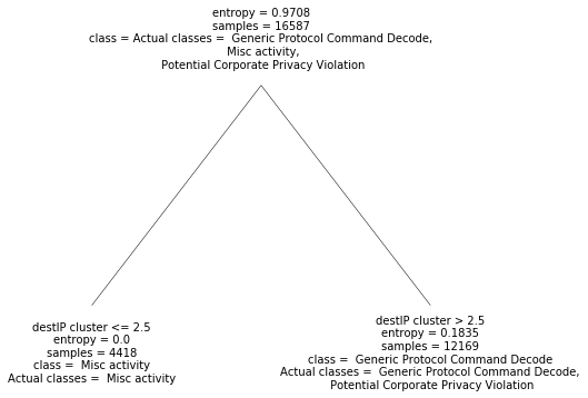
By default, entropy criterion is selected to initialise the decision tree and the flag of post-pruning is set as True. The cluster dataset generated before is firstly splitted into training set and test set randomly. Then the training set is fed to the decision tree then the decision tree is learned automatically. The final decision tree in text is shown below and it can also be illustrated in the Figure.
importrandomdeftrain_test_split(df,test_size):"""Split the data into train and test parts randomly.
Parameters:
df : pd.DataFrame, input data
test_size : either a percentage or the number of the test samples
Returns:
train_df : pd.DataFrame, training data
test_df : pd.DataFrame, test data
"""ifisinstance(test_size,float):test_size=round(test_size*len(df))indices=df.index.tolist()test_indices=random.sample(population=indices,k=test_size)test_df=df.loc[test_indices]train_df=df.drop(test_indices)returntrain_df,test_df
1
2
3
4
5
6
7
8
9
10
importrandomrandom.seed(1)# For reproductiontrain_data,test_data=train_test_split(cluster_data,test_size=0.1)dt=DesicionTree(post_prune=True)dt.feed(train_data)dt.view(method='t',saveflag=True)# View in textdt.view('g',True,savename='q5-decision-tree')# View in graph
Visulising the decision tree in text.
|---destIP cluster <= 2.5
| |--- Misc activity
|---destIP cluster > 2.5
| |--- Generic Protocol Command Decode
Visulising the decision tree graphically.
It is noticeable that although three classes (Generic Protocol Command Decode, Misc activity, Potential Corporate Privacy Violation) exist in the original training data, the only two son nodes predicts only two classes (Generic Protocol Command Decode, Misc activity) among the three. The decision tree can give a fairly certain ansewr in two cases.
This situation can be indicated by printing the confusion matrix while testing the decision tree. The test set is input to the predict function and a list of predicted classes is generated. I made use of both the ground truth classes and the predicted classes to produce the confusion matrix and print the precision, recall of the classification, shown as below. Obviously, all samples with class Potential Corporate Privacy Violation are the unseen data.
 1
 2
 3
 4
 5
 6
 7
 8
 9
10
11
12
13
14
15
16
17
18
extended_test_data=test_data.copy()# Deep copy to avoid shared referencepredicted_classes=dt.predict(extended_test_data)# Predictextended_test_data['predicted']=predicted_classes# Add a column of predictedfromsklearnimportmetricsy_true=extended_test_data['class'].to_numpy()y_predicted=extended_test_data['predicted'].to_numpy()# Classification reportprint('Classification report:\n',metrics.classification_report(y_true,y_predicted))# Confusion matrixprint('Confusion matrix:\n',metrics.confusion_matrix(y_true=y_true,y_pred=y_predicted))